The program is intended to be used to find interesting rules. It does this by generating random rule parameters and then running the resulting rule starting with a randomly generated pattern. This process is controlled by simply clicking a New Rule menu button. Options specifying how the rule parameters are to be modified are provided.
Patterns generated by running a CA simulation can be saved to and loaded from pattern files. These pattern files are compatible with MCell's pattern files (*.mcl) and can be used without change on both Square Cell and MCell.
The program provides controls which can be used to edit the CA simulation display and analyze the simulation patterns.
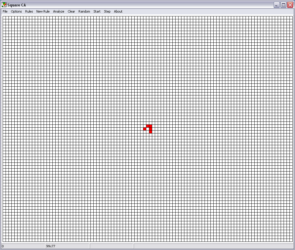
The program's main display is shown below.
The program will execute on a PC running Windows XP, is written in Delphi 5 and uses the Graphics32 library.
To get started, execute the program and click the menu item 'Rules | Load Rule'. This will display the Load Rule dialog shown below.
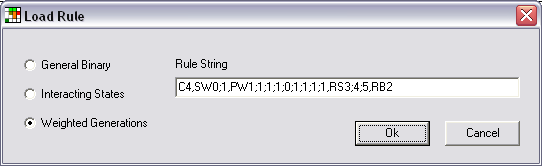
Notice that the Weighted Generations radio button is selected and that the Rule String edit control contains a default rule string. This rule string specifies the well known Star Wars rule. Click OK to select this default rule. Now click the Random menu to set the cells to random states and click the Start menu to run the simulation. Stop the simulation by clicking the Stop menu and step the simulation by clicking the Step menu. Clear the display by clicking the Clear menu. This sets the state of each cell to 0.
Now click Start and repeatedly click New Rule. This simple process together with setting new rule options, described below, randomly selects new rules in the Weighted Generations rule family and runs them.
Return to the Load Rule dialog and repeat this process using the default rules for the Interacting States and General Binary rule families.
Cell patterns may be saved to a pattern file by clicking 'File | Save' and restored from a pattern file by clicking 'File | Open'. The pattern files contain the rule string and the collection of cell states. The files are compatible with MCell. Try running a file generated by Square Cell in MCell and a file generated by MCell in Square Cell.
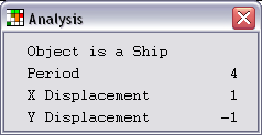
Cell patterns may be analyzed to determine if they are ships, oscillators or are stable. The message box shown below displays the result after clicking the Analyze menu button with Conway's well known glider displayed.
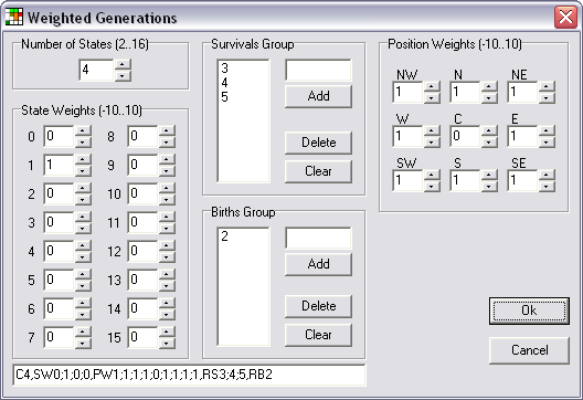
Each cell can be in one of 16 possible states in the range 0..15. Each iteration, the states of a cells 8 neighbors are multiplied by appropriate State and Position Weights and then counted. For example, if the NW neighbor is in state 3 and the State Weight corresponding to state 3 is 5 and the NW Position Weight is 2 then the NW neighbor will contribute a count of 10 (5 * 2) to the cells neighbor count. Both the State and Position Weights are in the range -10..10. If the C Position Weight is non zero then the cell may contribute to its own neighbor count. For example if the C Position Weight is -3 and the cell is in state 2 and the State Weight corresponding to state 2 is 3 then the cell's neighbor count will be decremented by 9 (3 * -3).
If a cell is in state 0 then it changes to state 1 if its neighbor count is included in the Birth Group. Otherwise the cell remains in state 0. If a cell is in state 1 then it remains in state 1 if its neighbor count is included in the Survival Group. If a cell is in state 1 and the cell's neighbor count is not included in the Survival Group and the number of states is greater than 2 then the cell's state changes to state 2, otherwise it changes to state 0. If a cell is in state n where n >= 2 and the number of states is s, then it changes to state n + 1 if n + 1 < s, otherwise the cell returns to state 0.
The Number of States, the State Weights and the Position Weights are modified by clicking the associated up or down arrow controls. The Birth and Survival Groups are provided with edit and button controls to add, delete and clear entries.
In the example shown above, the input dialog is set for the well know Star Wars rule.
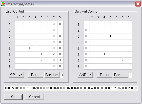
Each cell can be in one of 9 possible states in the range 0..8. On each iteration, the states of a cell's 8 neighbors are counted and the cell changes state according to the resulting count. If a cell is in state 0, it changes to a state in the range 1..8 if one or more of the conditions specified in the Birth Control is satisfied. Similarly, if a cell is not in state 0, it remains in its current state or returns to state 0 according to the conditions specified in the Survival Control. In the example input dialog shown above the settings in row 1 of the Birth Control state:
The Survival Control grid also has 8 rows. Each row contains settings which specify the conditions that must be satisfied for a cell to remain in state n where n is the row number. Again, if no condition is satisfied, the cell returns to state 0.
Grid values are changed by simply clicking them. Each click rotates the value through the range 0..8, incrementing with normal clicks and decrementing if the 'Shift' key is down.
Notice the two buttons labeled 'OR >=' and 'AND ='. These are toggle buttons which rotate through the values 'OR >=', 'OR =', 'AND >=' and 'AND ='. To see the relevance of these buttons carefully study the example described above.
For convenience, buttons are provided to reset each grid and to randomly select candidate conditions. Each of the random select buttons has an associated control which limits the generated counts. When clicked, these random select buttons generate two random numbers in the range 0..limit for each row and stores them in two random positions in that row. The limit values are changed in a manner similar to the grid values.
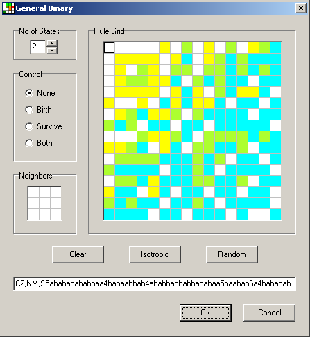
The General Binary rule contains specific specifications for a cell's behaviour based on the cell's neighbors that are in state 1. Display the General Binary dialog and click several squares in the Rule Grid. Notice that the pattern of pink squares in the Neighbor group changes with each click and that the radio button setting in the Control group also changes. The pink squares in the Neighbor group represent the pattern of neighbors that are in state 1 while the white squares represent neighbors that are not in state 1. There are 256 squares in the Rule Grid, one for each possible pattern of neighbors that are in state 1. Notice also, that the squares in the Rule Grid are colored white, cyan, yellow and green and that the selected radio button is related to the color of the square that is clicked. White squares select the radio button labeled None, cyan squares select Birth, yellow squares select Survive and green squares select Both.
Consider first the situation where the No of States is set to 2. On each iteration, the states of a cell's neighbors are examined and the pattern of neighbors in state 1 is determined. If a cell is in state 0 and the square in the Rule Grid corresponding to the cell's neighbor pattern is Birth (cyan) or Both (green) then the cell's state changes to 1, otherwise the cell remains in state 0. If a cell is in state 1 and the square in the Rule Grid corresponding to the neighbor pattern is Survive (yellow) or Both (green) then the cell remains in state 1, otherwise the cell changes to state 0.
Consider now the situation where the No of States is set to a value in the range 3..16. If a cell is in state 0 and the square in the Rule Grid corresponding to the cell's neighbor pattern is Birth (cyan) or Both (green) then the cell's state changes to 1, otherwise the cell remains in state 0. If a cell is in state 1 and the square in the Rule Grid corresponding to the neighbor pattern is Survive (yellow) or Both (green) then the cell remains in state 1. If a cell is in state 1 and the square in the Rule Grid corresponding to the neighbor pattern is not Survive (yellow) or Both (green) and the number of states is greater than 2 then the cell's state changes to state 2, otherwise it changes to state 0. If a cell is in state n where n >= 2 and the number of states is s, then it changes to state n + 1 if n + 1 < s, otherwise the cell returns to state 0.
A square in the Rule Grid can either be selected by clicking it directly or by clicking squares in the Neighbor group. In the later case clicking squares in the Neighbor group toggles their color between pink and white. When a square in the Rule Grid has been selected, it can be changed by selecting the appropriate radio button in the Control group.
Rules can be made isotropic by clicking the button labeled Isotropic. Under such rules, the evolution of cell patterns behaves the same regardless of pattern orientation. Cell patterns will evolve in the same manner if they are rotated through 90, 180 or 270 degrees or reflected about the X or Y axis.
A groups of cells is selected by clicking the display with the 'Ctrl' key down. The first click marks a corner of the area to be selected and the second click marks an opposite corner. A third click clears the selection. A selected cell groups may be manipulated by controls on the Selection Control popup dialog shown below. This dialog is displayed by Right clicking the display.
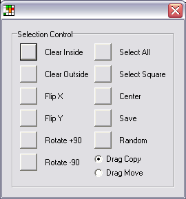
The cells inside the selecting rectangle may be set to state 0 by clicking the Clear Inside button. Similarly, the cells outside this rectangle may be set to 0 by clicking the Clear Outside button. Selected cell groups may be flipped about the X or Y axis or rotated through 90 degrees. All the cells that are not in state 0 may be selected by clicking the Select All button. As a convenience for group rotation, all cells that are not in state 0 may also be selected by surrounding them with a square by clicking the Select Square button. Control buttons are also provided to center the selected group of cells, set the selected cell states to randomly generated values and save the selected cells in a pattern file. Selected cell groups may be moved or copied by dragging them. The setting of the two radio buttons on the Selection Control dialog specify which function is active.
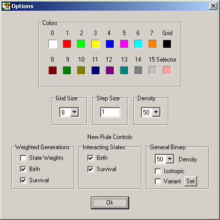
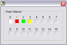
Each of the colors associated with the cell states, the cell grid and the cell group selector can be changed. Simply click on the appropriate square to display the color selector and choose a color.
The cell size in pixels can be set to any number in the range 1..15 using the Grid Size selector.
The number of simulation steps executed when the Step menu is clicked can be set using the Step Size edit control.
When either the display cells or a selected group of cells are set to random states (colors), the cell density can be set using the Density selector.
There are New Rule options available for each of the rule families supported.
For the Weighted Generations family, the new rule function generates random State Weights, random Birth Counts and random Survival Counts according to the settings of the check boxes. If a check box is checked, random values are generated and replace the current values and if the check box is not checked the current values are unchanged.
The new rule function for the Interacting States family works in a similar way. In this case two check boxes control the generation of random values for the Birth grid and the Survival grid. It is common to first check Birth and uncheck Survival and click the New Rule menu repeatedly until an interesting rule is found and then uncheck Birth and check Survival to explore variations of this rule.
The new rule options provided for the General Binary rule family consist of a Density selector, an Isotropic check box and a Variant check box and Set button. The Density selector specifies the approximate density of the random values generated to fill the Rule Grid. For example, if the density is set to 50% then half of the squares will be set to None and the other half will be evenly distributed between Birth, Survive and Both. The Isotropic check box simply specifies whether the new rule will be isotropic or not. If the variant Set button is clicked, the current rule settings are saved as a new base rule. If subsequently the Variant check box is checked, then the new rule function first loads the base rule and then modifies it. In this situation it is usual to set the Density to a small percentage.